Transfer Excel Data Between Sheets Automatically with Formulas

Managing data in Excel can be a tedious task, especially when you're dealing with large sets of information spread across multiple sheets. Fortunately, Excel provides powerful tools to make this process more efficient. In this post, we'll explore how to transfer Excel data between sheets automatically using formulas, offering you a method to streamline your work and reduce manual input.
Understanding the Basics
Before we dive into the specifics of transferring data, it's crucial to understand some foundational concepts:
- Cell References: Excel uses cell references to locate data within sheets.
- 3D References: A way to reference the same cell or range across multiple sheets.
- Named Ranges: Defines a name for a cell or range to simplify referencing.
Automatic Data Transfer with Formulas

The process of automatically transferring data from one sheet to another involves using formulas that dynamically pull information:
Using the VLOOKUP or INDEX-MATCH Functions

The VLOOKUP and INDEX-MATCH functions are Excel's workhorses for looking up values and pulling them from other locations. Here's how to use them:
=VLOOKUP(lookup_value, table_array, col_index_num, [range_lookup])
- lookup_value: The value you want to find.
- table_array: The range of cells that contains the data.
- col_index_num: The column number in the table_array from which to retrieve the value.
- [range_lookup]: TRUE for an approximate match, FALSE for an exact match (Optional).
📝 Note: VLOOKUP searches for the lookup_value in the first column of the table_array.
For INDEX-MATCH, which provides more flexibility:
=INDEX(return_array, MATCH(lookup_value, lookup_array, [match_type]))
- return_array: The range of cells from where to return the result.
- lookup_value: The value you're looking for.
- lookup_array: The range of cells to search for the lookup_value.
- [match_type]: 1 for less than, 0 for exact match, -1 for greater than (Optional).
Dynamic 3D References

3D references can be used to pull data from the same cell across multiple sheets. Suppose you want to gather data from cells A1 of sheets Sheet1, Sheet2, and Sheet3 into cell B1 of a summary sheet:
=AVERAGE(Sheet1:Sheet3!A1)
This formula calculates the average of cell A1 from the specified sheets.
Using Cell References Across Sheets

Direct cell references allow you to link cells from one sheet to another:
=Sheet1!A1
This formula pulls data from cell A1 in Sheet1 into any cell in another sheet.
Advanced Data Transfer Techniques

Named Ranges for Clarity
Creating named ranges can make your formulas cleaner and more understandable:
- Select the range you want to name.
- Go to the Formulas tab and choose "Define Name."
- Enter a meaningful name and click OK.
Now, you can use this named range in your formulas:
=SUM(MyRange)
📝 Note: Named ranges make your formulas more readable and easier to maintain.
Using Indirect Function for Flexible Referencing

The INDIRECT function turns a text string into a cell reference:
=INDIRECT("'Sheet1'!A1")
This function allows dynamic referencing, making it easier to build adaptable formulas.
Practical Examples

Example 1: Sales Data Consolidation
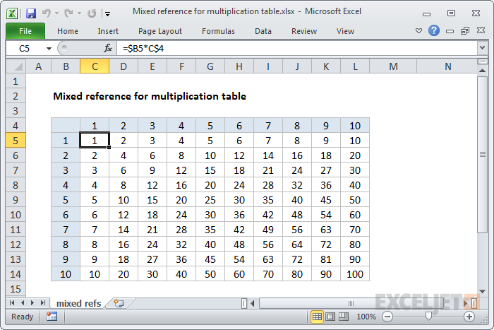
Imagine you have sales data spread across multiple sheets named by month:
| Sheet Name | Reference Cell | Formula |
|---|---|---|
| January | A1 | =January!A1 |
| February | A1 | =February!A1 |
| Summary Sheet | A1 | =SUM(January:December!A1) |
Example 2: Project Tracker
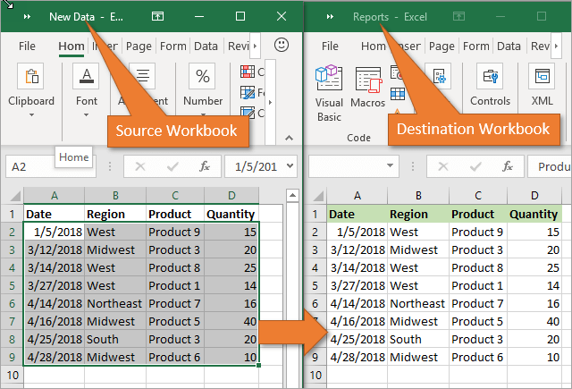
Suppose you have a project tracker with different statuses in different sheets:
- Sheet1: In Progress
- Sheet2: Pending Review
- Sheet3: Completed
To pull the status from these sheets into a master sheet:
=IF(ISBLANK(Sheet1!A1), "", Sheet1!A1)
=IF(ISBLANK(Sheet2!B1), "", Sheet2!B1)
=IF(ISBLANK(Sheet3!C1), "", Sheet3!C1)
Key Takeaways

Excel’s flexibility lies in its ability to automate data manipulation across sheets. By using formulas like VLOOKUP, INDEX-MATCH, named ranges, 3D references, and INDIRECT, you can create dynamic, interlinked spreadsheets that save time and reduce errors. Remember:
- Always check the accuracy of cell references and ensure they are updating as expected.
- Consider the performance impact of complex formulas, especially with large datasets.
- Regularly review and update your formulas to reflect changes in your data structure.
How can I dynamically reference a cell that might not exist in all sheets?

+
Use the IFERROR function to handle cells that don’t exist. For example: =IFERROR(Sheet1!A1, “”) returns an empty string if A1 does not exist in Sheet1.
Can I use these formulas for multiple columns of data at once?

+
Yes, by adjusting your range references in the VLOOKUP or INDEX-MATCH functions, you can dynamically pull data from multiple columns.
What is the advantage of using named ranges in Excel?

+
Named ranges make formulas more readable and easier to maintain. They also ensure consistency when referencing data from different sheets or parts of your workbook.