Find Duplicates In Excel Two Columns

Introduction to Finding Duplicates in Excel

When working with large datasets in Excel, it’s common to encounter duplicate values. These duplicates can be in a single column or across multiple columns. Finding and managing these duplicates is crucial for data accuracy and efficiency. This guide will focus on finding duplicates in two columns in Excel, a task that can be accomplished using various methods, including formulas, conditional formatting, and Excel’s built-in tools.

Understanding Duplicates in Excel

Duplicates in Excel refer to rows or cells that contain the same value or combination of values. When dealing with two columns, a duplicate is considered when the combination of values in both columns matches another row’s combination. For example, if you have a list of names and email addresses, a duplicate would be another row with the same name and email address.

Method 1: Using Conditional Formatting

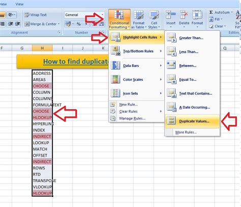
Conditional formatting is a powerful tool in Excel that allows you to highlight cells based on specific conditions, including duplicates. Here’s how to use it to find duplicates in two columns: - Select the range of cells across the two columns you want to check for duplicates. - Go to the “Home” tab on the Ribbon. - Click on “Conditional Formatting” and then select “Highlight Cells Rules” > “Duplicate Values”. - In the dialog box, you can choose the formatting you want to apply to the duplicates. - Click “OK” to apply the formatting.

This method will highlight all duplicate combinations in the selected range but won’t remove them. It’s useful for visually identifying duplicates.

Method 2: Using Formulas

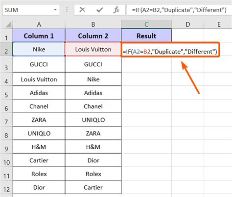
You can use a formula to identify duplicates in two columns. The COUNTIFS function is particularly useful for this purpose: - Assume your data is in columns A and B, starting from row 1. - In a new column (say, column C), enter the following formula in the first row of your data (C1):

=COUNTIFS(A:A, A1, B:B, B1) > 1

• Drag the formula down to apply it to all rows.
• This formula returns TRUE if the combination in columns A and B is a duplicate and FALSE otherwise.

You can then filter on this column to show only the duplicates.

Method 3: Using Excel’s Remove Duplicates Feature

Excel has a built-in feature to remove duplicates, which can also be used to identify them: - Select the range of cells including the header row. - Go to the “Data” tab on the Ribbon. - Click on “Remove Duplicates”. - In the Remove Duplicates dialog box, select the columns you want to consider for duplicate removal. - Before clicking “OK”, make sure to check the box that says “My data has headers” if your range includes headers. - Instead of clicking “OK” to remove duplicates, click “Cancel” and then apply a filter to your data to highlight duplicates, or proceed with removing them if that’s your intention.

Method 4: Using PivotTables

PivotTables can also be used to identify duplicates by counting the occurrences of each combination: - Select your data range. - Go to the “Insert” tab and click on “PivotTable”. - Choose a cell to place your PivotTable and click “OK”. - Drag one of your columns to the “Row Labels” area and the other to the “Row Labels” as well, so both are listed. - Then, drag any field to the “Values” area. It doesn’t matter which field you choose since we’re just using it to count occurrences. - Right-click on the field in the “Values” area and select “Value Field Settings”. - Change the value field setting to “Count” and click “OK”.

This method gives you a count of each unique combination and can help in identifying duplicates by showing which combinations occur more than once.

Method 5: Using VBA Macro

For those comfortable with VBA, you can write a macro to find duplicates:

Sub FindDuplicates()
    Dim ws As Worksheet
    Set ws = ThisWorkbook.Sheets("Sheet1") 'Change to your sheet name
    
    Dim rng As Range
    Set rng = ws.Range("A1:B" & ws.Cells(ws.Rows.Count, "A").End(xlUp).Row)
    
    rng.RemoveDuplicates Columns:=Array(1, 2), Header:=xlYes
End Sub

This macro removes duplicates based on columns A and B. You can modify it to simply highlight duplicates by iterating over the range and checking for duplicates instead of removing them.

📝 Note: When using any method to identify or remove duplicates, ensure you have a backup of your original data to avoid losing important information.

To summarize, finding duplicates in two columns in Excel can be efficiently done using conditional formatting for a quick visual check, formulas for more detailed analysis, Excel’s built-in remove duplicates feature, PivotTables for a summary view, or VBA macros for automation. Each method has its use case, and the choice depends on your specific needs and comfort level with Excel.